Open Access Monitoring with OpenAlex
Sophia Dörner 
This notebook is a tool for library and information professionals dealing with monitoring Open Access publication output at their institution. It shows how to leverage OpenAlex to retrieve and analyze publication data using R. No software installation or prior programming knowledge required. At the end of the notebook you will find some short excercises that can be executed directly in your browser. If you have suggestions or notice any mistake, please open an issue.
What is OpenAlex?
OpenAlex is a fully-open bibliographic database operated by the non-profit organization OurResearch. It launched in 2022 as a successor to the then discontinued Microsoft Academic Graph (Priem et al., 2022). OpenAlex data comprises information about various entities of the scholarly ecosystem such as research outputs (journal articles, books, datasets, etc.), authors, sources, etc. (OurResearch, n.d.).
The OpenAlex dataset is a useful tool to monitor open access activities on different levels of aggregation, as OpenAlex e.g. provides information on the open access status of a work or information on estimates for article processing charges (APCs) at the journal and work levels.
How can I access OpenAlex data?
OpenAlex offers three main ways to access the data:
The OpenAlex web user interface
In the web user interface you are able to query the database via a search bar, apply filters and export the results in csv, ris or txt format.
The OpenAlex API
The OpenAlex REST API allows programmatic access to and retrieval of OpenAlex data1. To interact with the API you are required to register an API key as of February 2026 (Priem, 2026). The API is designed as a freemium service; more detailed information on the pricing model is provided in the OpenAlex technical documentation. However, the free daily quota is sufficient for our use case in this notebook.
OpenAlex API Key
To get your free API key you need to:
- Create a free account at openalex.org
- Copy your API key from https://openalex.org/settings/api
Best coding practice is to store credentials in your .Renviron file. To add your API Key to the .Renviron file you go into the console and type:
file.edit("~/.Renviron")The file opens and you can store your OpenAlex API Key by typing:
openalexR.apikey = YOUR_API_KEYThen you need to save the file and are good to go.
The OpenAlex data snapshot
OpenAlex additionally offers a data snapshot with a copy of the complete database for download, which a user can then load into their own data warehouse or relational database. The snapshot gets updated monthly.
Exploring OpenAlex institutional open access data
In this notebook we will query the OpenAlex API with R (R Core Team, 2025) to answer the following question:
How many of recent journal articles from a given institution are open access and how did the share of open access publications evolve over the years?
To answer the question, we will filter OpenAlex work records to be:
- of type article
- have at least one author affiliated with a specific institution (the notebook uses the example of the University of Göttingen)
- published between 2020 and 2024
and we will limit the number of fields (or columns) returned by the API to:
- the OpenAlex ID associated with the article
- the digital object identifier (DOI) of the article
- the title of the article
- the publication year of the article
- journal information
- open access information
- information on the apc list prices and
- information on the paid apc prices
OpenAlex offers a lot more information than what we are exploring in this notebook. For a full documentation of all available entities and fields, please visit the OpenAlex technical documentation.
Loading packages
We will load the openalexR package (Aria et al., 2024) that allows us to query the OpenAlex API from within our notebook. We will also load the packages dplyr (Wickham et al., 2023), tidyr (Wickham et al., 2024), stringr (Wickham, 2025) and ggplot2 (Wickham, 2016) that provide a lot of additional functionalities for data wrangling and visualization and are part of the tidyverse package (Wickham et al., 2019).
Loading data
We won’t query the API in this notebook directly. We ran the API query once and stored the results in a separate file we will load into the notebook in a following code chunk.
We will use the oa_fetch function from the openalexR package to query the OpenAlex API and store the returned tibble (a data frame that works well with the tidyverse) in the object df.
df <- openalexR::oa_fetch(
  entity = "works",
  institutions.ror = "01y9bpm73", # change the ROR id if you want to analyse the performance of another institution
  type = "article",
  is_paratext = FALSE,
  is_retracted = FALSE,
  from_publication_date = "2020-01-01",
  to_publication_date = "2024-12-31",
  options = list(select = c(
    "id", "doi", "title", "publication_year",
    "primary_location", "open_access", "apc_list", "apc_paid"
  )),
  output = "tibble",
  paging = "cursor",
  abstract = FALSE
)
We have saved the query result as an rds-file, which we will now load. You can skip this step if you have adapted the notebook to investigate the publication output of your institution.
df <- readRDS("notebooks/openalex_data.rds")Structure of the dataset
To get an overview of the structure of our data frame, especially the number of rows (observations) and columns (variables), the individual column names and the data types they contain, we will use the glimpse function from the dplyr package, which is part of the tidyverse.
dplyr::glimpse(df)Rows: 15,952
Columns: 19
$ id <chr> "https://openalex.org/W3009912996", "https…
$ title <chr> "SARS-CoV-2 Cell Entry Depends on ACE2 and…
$ doi <chr> "https://doi.org/10.1016/j.cell.2020.02.05…
$ publication_year <int> 2020, 2021, 2020, 2020, 2020, 2020, 2020, …
$ is_oa <lgl> TRUE, FALSE, TRUE, TRUE, TRUE, TRUE, TRUE,…
$ is_oa_anywhere <lgl> TRUE, TRUE, TRUE, TRUE, TRUE, TRUE, FALSE,…
$ oa_status <chr> "bronze", "green", "bronze", "hybrid", "hy…
$ oa_url <chr> "https://www.cell.com/article/S00928674203…
$ any_repository_has_fulltext <lgl> TRUE, TRUE, TRUE, TRUE, TRUE, FALSE, FALSE…
$ source_display_name <chr> "Cell", "Diabetes Research and Clinical Pr…
$ source_id <chr> "https://openalex.org/S110447773", "https:…
$ issn_l <chr> "0092-8674", "0168-8227", "1097-2765", "00…
$ host_organization <chr> "https://openalex.org/P4310315673", "https…
$ host_organization_name <chr> "Cell Press", "Elsevier BV", "Elsevier BV"…
$ landing_page_url <chr> "https://doi.org/10.1016/j.cell.2020.02.05…
$ pdf_url <chr> "https://www.cell.com/article/S00928674203…
$ license <chr> "other-oa", NA, "other-oa", "cc-by", "cc-b…
$ version <chr> "publishedVersion", NA, "publishedVersion"…
$ apc <list> [<data.frame[2 x 5]>], [<data.frame[2 x 5…The output shows that our data frame contains a total of 15,952 rows (observations) and 19 columns. Furthermore, it shows that most of the column values are of data type character (chr), the publication year column values are of type integer (int), some of the open access column values are of type logical (lgl) and the apc column values are of type list (list). The output also indicates the first values of every column on the right hand side.
The first values show us two important things:
- There are at least some missing values within our data frame as is indicated by the NA in the license and version columns. NA is not a common string or numeric value, but a reserved word in R for the logical constant which contains a missing value indicator, i.e. R uses NA to indicate that the specific value is missing.
- The apc column contains data frames as values. This means we can’t access the apc information directly. We will explore later in the notebook how to transform the column and access the apc information.
To look at the first 10 rows of our data frame we are using the head function.
head(df, 10)# A tibble: 10 × 19
id title doi publication_year is_oa is_oa_anywhere oa_status oa_url
<chr> <chr> <chr> <int> <lgl> <lgl> <chr> <chr>
1 https://o… SARS… http… 2020 TRUE TRUE bronze https…
2 https://o… IDF … http… 2021 FALSE TRUE green https…
3 https://o… A Mu… http… 2020 TRUE TRUE bronze https…
4 https://o… Neur… http… 2020 TRUE TRUE hybrid https…
5 https://o… COVI… http… 2020 TRUE TRUE hybrid https…
6 https://o… Olfa… http… 2020 TRUE TRUE hybrid https…
7 https://o… Mana… http… 2020 TRUE FALSE closed https…
8 https://o… SARS… http… 2021 TRUE TRUE green https…
9 https://o… Infe… http… 2020 TRUE TRUE hybrid https…
10 https://o… The … http… 2021 TRUE TRUE bronze https…
# ℹ 11 more variables: any_repository_has_fulltext <lgl>,
# source_display_name <chr>, source_id <chr>, issn_l <chr>,
# host_organization <chr>, host_organization_name <chr>,
# landing_page_url <chr>, pdf_url <chr>, license <chr>, version <chr>,
# apc <list>The first argument within the head function is our data frame df and the second argument is the number of rows we want to have returned. Each row within our data frame corresponds to an article.
Data wrangling with the tidyverse
Before analysing the OpenAlex data, we will have a closer look at the publisher and apc columns and perform some data wrangling tasks.
To get an overview of the publishers present in our dataframe and the number of articles per publisher, we will use three tidyverse functions and the base R pipe operator |>. The magrittr package, which is part of the tidyverse, provides another pipe operator (%>%), however, we will use the base R pipe since you won’t need to install an additional package to use it.
The pipe operator allows us to take e.g. a data frame or the result of a function and pass it to another function. If we type the name of our data frame followed by the pipe operator that means we don’t have to specify which data we want a function to be performed on, when we call it after the pipe operator.
The group_by function allows us to group data in our data frame df by one or more variables. In this case we will group the data frame by the OpenAlex provided id for the publisher in our host_organization column and the publisher name in our host_organization_name column. This allows us to generate aggregate statistics for the publishers in our data frame.
The summarise function allows us to calculate summary statistics for each group. In this case we will use the n function to count the number of observations in each group, and the result is stored in a new variable called n.
The arrange function is used to sort the data based on the n variable and the desc function lets us determine that the ordering should be in descending order. This means that the groups with the highest number of observations will appear at the top of the output.
# A tibble: 443 × 3
# Groups:   host_organization [443]
   host_organization                host_organization_name                     n
   <chr>                            <chr>                                  <int>
 1 https://openalex.org/P4310320990 Elsevier BV                             2506
 2 https://openalex.org/P4310320595 Wiley                                   2121
 3 https://openalex.org/P4310319900 Springer Science+Business Media         1395
 4 <NA>                             <NA>                                    1127
 5 https://openalex.org/P4310310987 Multidisciplinary Digital Publishing …  1073
 6 https://openalex.org/P4310319908 Nature Portfolio                         650
 7 https://openalex.org/P4310320527 Frontiers Media                          506
 8 https://openalex.org/P4310311648 Oxford University Press                  481
 9 https://openalex.org/P4310319965 Springer Nature                          417
10 https://openalex.org/P4310320006 American Chemical Society                388
# ℹ 433 more rows
The output shows us some important things about the data:
- There is a significant amount of articles that don’t have any publisher assigned. We can’t cover data cleaning tasks in-depth in this notebook but want to point out that this is something worth investigating further. Questions that could be asked are: Do these articles have a DOI? Were these articles misclassified in any way? Did the publisher information get lost for some reason? Are there any other inconsistencies with these articles? Can I disregard some or all of the articles?
- Publisher names are at least in some cases not standardized or aggregated to a single publishing house. The approach taken to represent the publishing structure, i.e. listing imprints or subsidiaries separately or under the main publisher name, and the point in time of the analysis, have an influence of the results, e.g. because of changes in ownership (see also Scheidt, 2025).
As an example we will look at the publisher names in our data frame that contain Springer or Nature. We will use the filter function from the tidyverse that lets us filter articles that fulfil the condition we specify in combination with the grepl function that allows to search for patterns. In this case we will use a regular expression as the pattern to search for.
# A tibble: 8 × 3
# Groups:   host_organization [8]
  host_organization                host_organization_name                n
  <chr>                            <chr>                             <int>
1 https://openalex.org/P4310319900 Springer Science+Business Media    1395
2 https://openalex.org/P4310319908 Nature Portfolio                    650
3 https://openalex.org/P4310319965 Springer Nature                     417
4 https://openalex.org/P4310319986 Springer VS                          28
5 https://openalex.org/P4310320108 Springer Nature (Netherlands)         9
6 https://openalex.org/P4310319972 Springer International Publishing     3
7 https://openalex.org/P4310321666 Springer Vienna                       2
8 https://openalex.org/P4310320090 Springer Medizin                      1
If we want to replace the Springer name variants with Springer Nature as publisher name, we can use the mutate function that lets us transform a column in our data frame in combination with the str_replace_all function that lets us replace string values that follow a pattern we specify to do so.
# A tibble: 434 × 2
   host_organization_name                             n
   <chr>                                          <int>
 1 Elsevier BV                                     2506
 2 Springer Nature                                 2505
 3 Wiley                                           2121
 4 <NA>                                            1127
 5 Multidisciplinary Digital Publishing Institute  1073
 6 Frontiers Media                                  506
 7 Oxford University Press                          481
 8 American Chemical Society                        388
 9 American Physical Society                        350
10 Taylor & Francis                                 326
# ℹ 424 more rows
Be aware that this data transformation only applies to the publisher name column and not the OpenAlex provided publisher id column. We would need to perform a separate transformation step to align both. Additionally, we did not permanently rename the publisher name values in our data frame. To do this we can either override our data frame df or create a new data frame by assigning the output with the <- operator.
# overriding our data frame
df <- df |>
  dplyr::mutate(host_organization_name = stringr::str_replace_all(host_organization_name, "^Springer.*$|Nature.*$", "Springer Nature"))

# creating a new data frame df2
df2 <- df |>
  dplyr::mutate(host_organization_name = stringr::str_replace_all(host_organization_name, "^Springer.*$|Nature.*$", "Springer Nature"))
To access the apc values in our data frame we will use the unnest_wider, unnest_longer, and pivot_wider functions from the tidyverse with the apc column.
The unnest_wider function allows us to turn each element of a list-column into a column. We will further use the select function to print only the resulting apc columns.
df |>
  tidyr::unnest_wider(apc, names_sep = ".") |>
  dplyr::select(starts_with("apc"))
# A tibble: 15,952 × 6
apc.type apc.value apc.currency apc.value_usd apc.provenance apc.1
<list<chr>> <list<dbl>> <list<chr>> <list<dbl>> <list<chr>> <lgl>
1 [2] [2] [2] [2] [2] NA
2 [2] [2] [2] [2] [2] NA
3 [2] [2] [2] [2] [2] NA
4 NA
5 [2] [2] [2] [2] [2] NA
6 [2] [2] [2] [2] [2] NA
7 NA
8 [2] [2] [2] [2] [2] NA
9 NA
10 [2] [2] [2] [2] [2] NA
# ℹ 15,942 more rowsThe output shows that the values in the apc columns are lists. This is because OpenAlex provides information for APC list prices and prices of APCs that were actually paid, when available. To transform the lists into single value cells we will use the unnest_longer function that does precisely that.
df |>
  tidyr::unnest_wider(apc, names_sep = ".") |>
  tidyr::unnest_longer(c(apc.type, apc.value, apc.currency, apc.value_usd, apc.provenance)) |>
  dplyr::select(id, starts_with("apc"))
# A tibble: 22,044 × 7
id apc.type apc.value apc.currency apc.value_usd apc.provenance apc.1
<chr> <chr> <dbl> <chr> <dbl> <chr> <lgl>
1 https://o… list 10100 USD 10100 <NA> NA
2 https://o… paid NA <NA> NA <NA> NA
3 https://o… list 3970 USD 3970 <NA> NA
4 https://o… paid NA <NA> NA <NA> NA
5 https://o… list 9080 USD 9080 <NA> NA
6 https://o… paid NA <NA> NA <NA> NA
7 https://o… list 3690 EUR 4790 <NA> NA
8 https://o… paid 3690 EUR 4790 <NA> NA
9 https://o… list 9750 EUR 11690 <NA> NA
10 https://o… paid 9750 EUR 11690 <NA> NA
# ℹ 22,034 more rowsThe output shows that we now have multiple rows for the same id. To transform the data frame to single rows for each id we will use the pivot_wider function that allows us to increase the number of columns and decrease the number of rows.
df |>
  tidyr::unnest_wider(apc, names_sep = ".") |>
  tidyr::unnest_longer(c(apc.type, apc.value, apc.currency, apc.value_usd, apc.provenance)) |>
  tidyr::pivot_wider(id_cols = id, names_from = apc.type, values_from = c(apc.value, apc.currency, apc.value_usd, apc.provenance))
# A tibble: 11,022 × 9
id apc.value_list apc.value_paid apc.currency_list apc.currency_paid
<chr> <dbl> <dbl> <chr> <chr>
1 https://op… 10100 NA USD <NA>
2 https://op… 3970 NA USD <NA>
3 https://op… 9080 NA USD <NA>
4 https://op… 3690 3690 EUR EUR
5 https://op… 9750 9750 EUR EUR
6 https://op… 10100 NA USD <NA>
7 https://op… 10100 NA USD <NA>
8 https://op… 1800 1800 USD USD
9 https://op… 9750 9750 EUR EUR
10 https://op… 3920 3920 GBP GBP
# ℹ 11,012 more rows
# ℹ 4 more variables: apc.value_usd_list <dbl>, apc.value_usd_paid <dbl>,
# apc.provenance_list <chr>, apc.provenance_paid <chr>The output doesn’t show all 9 variables (or columns). Underneath the preview we get the information:
4 more variables: apc.value_usd_list
, apc.value_usd_paid , apc.provenance_list , apc.provenance_paid
This means that they are in fact available in our data frame but are omitted in the preview.
Now we can access the APC information provided by OpenAlex. In this notebook we won’t analyse APC information any further. If you are interested in APC analysis, we offer a notebook showing how to analyse APC information using the OpenAPC data set at: https://oa-datenpraxis.de/OpenAPC.html
Analysing institutional open access performance
In the following sections, we will analyse the data to address our question and generate visualizations. This notebook can’t provide an in-depth analysis, but it will demonstrate how to apply some useful functions from base R and the tidyverse to gain insights from the data and show how to create visualisations using the ggplot2 package (Wickham, 2016).
How many of the institutions publication are open access?
To determine total number of open access publications of the research organization, we are using the sum function on the is_oa column. This column contains boolean values (true or false) and the sum function will sum up all rows that contain true values.
sum(df$is_oa, na.rm = T)[1] 10668We also provided the na.rm=T argument to the sum function which causes NA values to be removed.
When we check for NA values in the is_oa column using the is.na function, we see that there are 21 articles where the open access status is not determined.
To determine the overall open access share over all publication years in our data frame, we divide the total number of open access publications by the total number of publications. We calculate the latter using the n_distinct function on our id column. The n_distinct function is quite handy as it returns the number of unique values in the provided column. Since we provide the id column, it will return the total number of publications in our data frame.
round(sum(df$is_oa, na.rm = T) / n_distinct(df$id) * 100, 2)[1] 66.88How are open access publications distributed across journals?
To analyse the distribution of open access articles across journals we will calculate the total number of articles (n_articles), the total number of open access articles (n_oa_articles) and the total number of closed articles (n_closed_articles) per journal. We will again use the group_by, summarise and arrange functions. However, since we noticed that 21 articles have an undetermined open access status, we will first filter out all rows with NA values in the is_oa column. We will also group the data by the source_display_name column to generate aggregate statistics for the journals.
# A tibble: 4,156 × 4
   source_display_name                n_articles n_oa_articles n_closed_articles
   <chr>                                   <int>         <int>             <int>
 1 Scientific Reports                        221           221                 0
 2 Astronomy and Astrophysics                219           215                 4
 3 Journal of High Energy Physics            173           173                 0
 4 Nature Communications                     170           170                 0
 5 PLoS ONE                                  124           123                 1
 6 The European Physical Journal C            97            97                 0
 7 Forests                                    95            95                 0
 8 Angewandte Chemie                         103            92                11
 9 International Journal of Molecula…         84            84                 0
10 <NA>                                      414            84               330
# ℹ 4,146 more rows
The results show that 414 articles have no journal assigned within our data frame. This could indicate that more data cleaning needs to be performed. The results further show that the top three journals in terms of open access publication volume are Scientific Reports, Astronomy and Astrophysics, and Journal of High Energy Physics.
We can further explore the open access status distribution for the articles. We will do this on the example of the top three journals in terms of open access publication volume.
# A tibble: 8 × 4
# Groups:   source_display_name, is_oa [4]
  source_display_name            is_oa oa_status     n
  <chr>                          <lgl> <chr>     <int>
1 Astronomy and Astrophysics     FALSE closed        1
2 Astronomy and Astrophysics     FALSE green         3
3 Astronomy and Astrophysics     TRUE  bronze       95
4 Astronomy and Astrophysics     TRUE  green         1
5 Astronomy and Astrophysics     TRUE  hybrid      119
6 Journal of High Energy Physics TRUE  diamond     168
7 Journal of High Energy Physics TRUE  green         5
8 Scientific Reports             TRUE  gold        221
The results show that there are some data inconsistencies for the Astronomy and Astrophysics journal regarding the green open access status. Furthermore Scientific Reports appears to be a true gold open access journal.
How does the number of open access publications evolve over time?
We can combine functions from the tidyverse and ggplot2 to visualise the development of open access over time.
First, we group the data by publication year and open access status. We will then compute the number of articles in each group. In the ggplot function, we assign the publication year column to the x axis and the number of articles to the y axis. We choose point (geom_point) and line (geom_line) graph types to mark the distinct values of n and have them connected by lines. Both are provided with a colour aesthetic which is set to our open access status column. This will result in different colours being assigned to the points and lines for the different open access status values. With the theme_minimal option we are applying a minimal theme for the plot appearance.
df |>
  dplyr::group_by(publication_year, oa_status) |>
  dplyr::summarise(n = n(), .groups = "keep") |>
  ggplot(aes(x = publication_year, y = n)) +
  geom_line(aes(colour = oa_status)) +
  geom_point(aes(colour = oa_status)) +
  theme_minimal()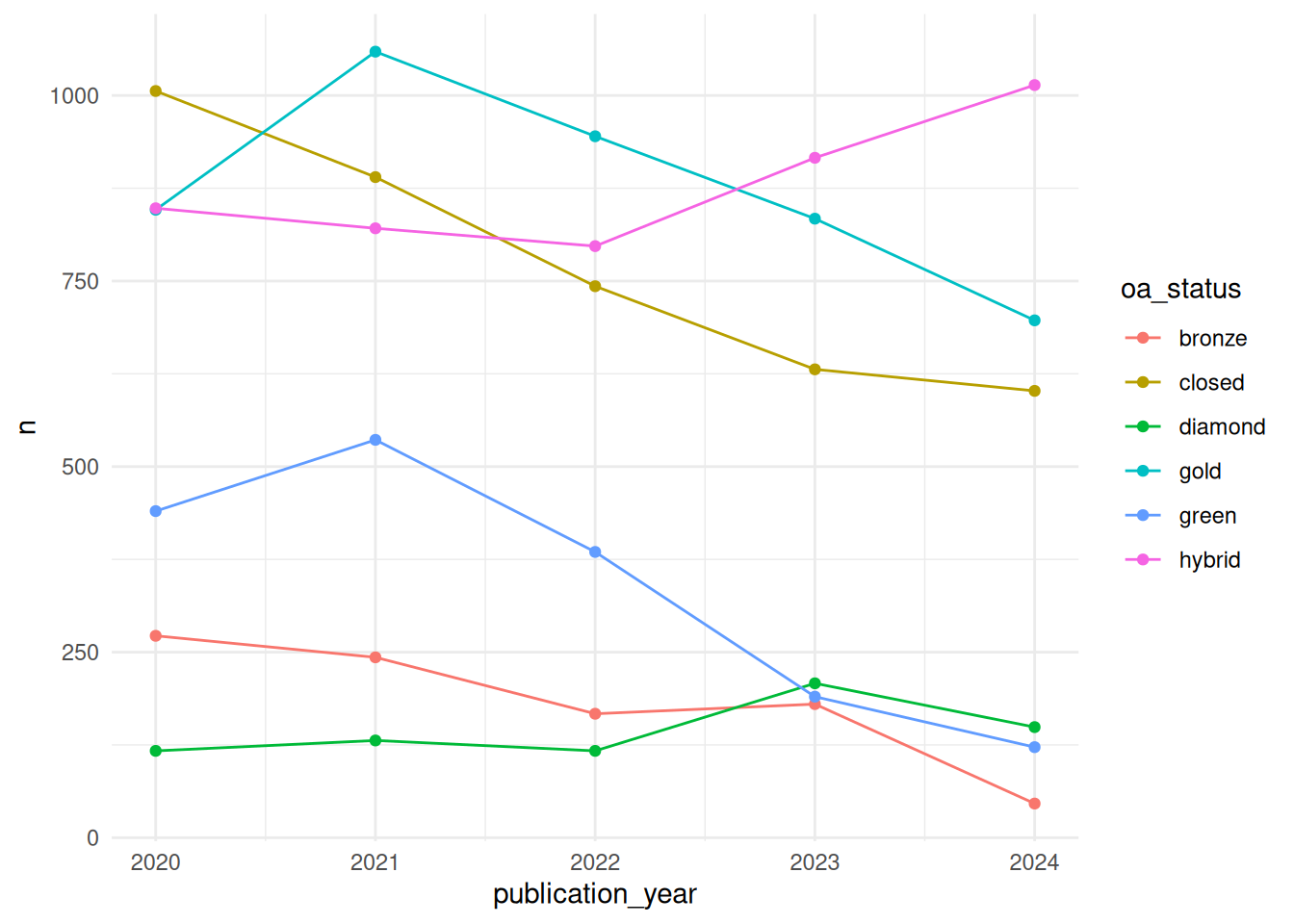
The plot shows use the total number of publications for each publication year and open access status. Generally, there seems to be a downwards trend in terms of publication volume for all open access status types but hybrid open access.
We can further choose to visualise the open access distribution over time in terms of percentages. For this we first calculate the share of each open access status per publication year and create a new column using the mutate function that stores these values. We pipe the result through to the ggplot function assigning the publication year column to the x axis and the share to the y axis. We assign the oa_status column to the fill argument which will plot a different colour for each open access status. For this plot we choose a bar chart (geom_bar) graph type and again apply the minimal theme.
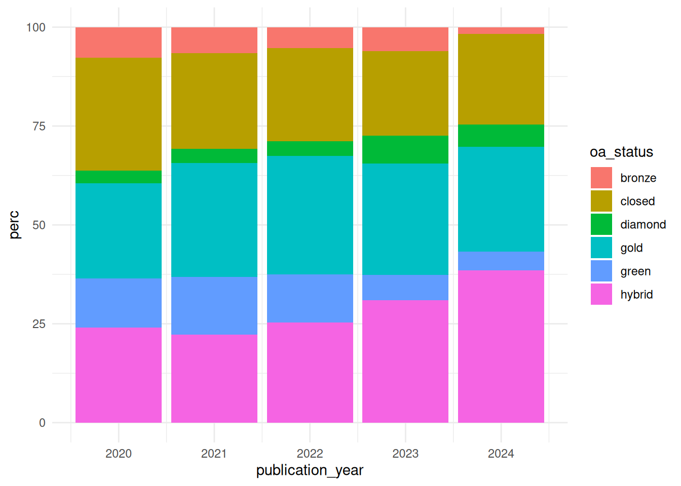
The plot shows use the share of each open access status for each publication year. The most dominant open access types are gold and hybrid open access. Furthermore the share of open access publications across all publication years is higher than for closed access publications.
Exercises
The following exercises focus on open access publications in regard to publishers and journals. The code is presented in interactive code blocks. You can adapt the code and run it by clicking on run code.
Aggregate statistics for publishers
Before, we analysed the distribution of open access articles across journals. Below is a copy of the corresponding code. Adapt the code to give you aggregate statistics for publishers instead of journals.
Which publishers are among the top three in terms of overall publication volume and in terms of open access publication volume? Do you notice any interesting patterns?
Visuzlisation of open access disctribution by top three publishers
Now, see if you can adapt the code we used to visualise the open access share over time to show you the open access share for the top three publishers in terms of open access publication volume.
Hint: You’ll want to change something in the code so that you filter first based on the publisher names of the top three publishers before you perform the grouping. You can reuse code that was already introduced in the notebook.
References
Footnotes
API stands for Application Programming Interface. An API call is a request made by a client to an API endpoint on a server to retrieve or send information. An API call is a way for different applications to communicate with each other. The client (e.g. you, the user) makes the request and the server sends back a response (e.g. the OpenAlex data you requested).↩︎